Rooftop Solar PV Capacity & Annual Energy Yield Estimator
Spatial solar engineering calculator computing installed DC peak capacity, annual alternating current electrical yield, module quantities, specific yield, carbon emissions offsets, and grid tension classifications.
Standard formulation where peak capacity P_dc scales by total annual irradiance and overall performance ratio PR.
Realistic operational range factoring thermal cell heating, inverter clipping, cabling resistance, and soiling.
Annual tilted plane irradiance across Southern Europe and Mediterranean solar basins.
Normalized Digital Surface Model isolating building heights and filtering out shadowed or over-steep roof planes.
Theoretical and Mathematical Foundation of Rooftop Solar Modeling
Estimating the electricity generation potential of a rooftop photovoltaic installation requires a rigorous mathematical bridge connecting structural civil geometry, semiconductor device physics, and local meteorological solar radiation regimes. A primary source of planning failure in regional renewable energy programs is treating gross rooftop polygon surface area as 100% usable photovoltaic aperture.
1. Standard Test Conditions (STC) and Peak DC Capacity
The nameplate capacity of a photovoltaic module is rated under internationally standardized laboratory conditions designated as Standard Test Conditions (STC):
- Irradiance ($G_{stc}$): $1,000\text{ W/m}^2$ normal to the module surface.
- Cell Junction Temperature ($T_{cell}$): $25^\circ\text{C}$.
- Solar Spectral Distribution: Air Mass $AM = 1.5$ global spectrum (IEC 60904-3).
Under STC, the conversion efficiency ($\eta_{module}$) of a module defines the ratio of electrical output to incident solar power:
P_dc (kWp) = Net Usable Area [m2] * (eta_module [%] / 100) * 1.0 kW/m2
For modern commercial monocrystalline passivated emitter and rear cell (PERC) or tunnel oxide passivated contact (TOPCon) modules, module conversion efficiency ranges between 20.0% and 22.5%. A net usable area of $100\text{ m}^2$ fitted with 21.0% efficient modules yields a peak nominal DC capacity of:
P_dc = 100 m2 * 0.210 * 1.0 kW/m2 = 21.0 kWp
2. The IEC 61724 Photovoltaic Performance Ratio (PR) Formulation
In outdoor operating conditions, solar modules never produce at 100% of their STC laboratory rating continuously. The standard IEC 61724 formulation for annual alternating current (AC) electrical yield ($E_{annual}$, expressed in kilowatt-hours) integrates incident plane-of-array irradiation ($G_{annual}$, in $\text{kWh/m}^2/\text{year}$) and the overall system Performance Ratio ($PR$):
E_annual (kWh/year) = P_dc [kWp] * (G_annual [kWh/m2/yr] / 1.0 kW/m2) * PR
The Performance Ratio ($PR$) represents the cumulative product of several distinct physical loss mechanisms:
PR = eta_temp * eta_inv * eta_cable * eta_soil * eta_mismatch * eta_lid
- Thermal Junction Derating ($\eta_{temp} \approx 0.88 - 0.92$): As solar irradiance heats the dark module face, cell temperature rises far above ambient air according to the Nominal Module Operating Temperature (NMOT/NOCT) model:
Because monocrystalline silicon possesses a negative power temperature coefficient of approximately $\gamma_{pmax} \approx -0.35\% / ^\circ\text{C}$, operating at $60^\circ\text{C}$ in Mediterranean summer heat reduces instantaneous electrical power output by $12.25\%$.
T_cell = T_ambient + G_poa * ((NOCT - 20) / 800) - Inverter Conversion Efficiency ($\eta_{inv} \approx 0.97 - 0.985$): Transformation of direct current (DC) into 50/60 Hz alternating current (AC) by modern transformerless string or central inverters.
- Ohmic Wiring Resistance ($\eta_{cable} \approx 0.98 - 0.99$): Joule losses ($I^2 R$) in DC solar string cables and AC interconnection conductors.
- Soiling and Dirt Accumulation ($\eta_{soil} \approx 0.95 - 0.98$): Atmospheric particulate matter, pollen, dust, and avian deposits obscuring the glass cover plate.
- Module Quality and Mismatch ($\eta_{mismatch} \approx 0.98 - 0.99$): Manufacturing tolerance deviations between series-connected modules within the same MPPT string.
3. Specific Yield and Carbon Offset Formulation
Specific Yield ($Y_f$, expressed in $\text{kWh/kW}_p/\text{year}$) evaluates system quality independent of physical size:
Specific Yield (Y_f) = E_annual [kWh] / P_dc [kWp]
Annual carbon dioxide emissions avoided ($CO_{2,\text{offset}}$ in metric tons per year) are computed by multiplying annual AC generation by the regional electrical grid carbon intensity factor ($EF_{grid}$, typically $0.380\text{ kg } CO_2 / \text{kWh}$ for the European Mediterranean grid average):
CO2 Offset (metric tons/yr) = (E_annual [kWh] * EF_grid [kg CO2/kWh]) / 1000
Grid Interconnection Voltage Tiers & Distribution System Architecture
Photovoltaic generation assets interface with electrical grids across standardized voltage classes defined by international standards (IEC 61724, EN 50549, and national distribution codes). The grid connection architecture dictates balance-of-system requirements, telemetry obligations, and transformer substation investments:
| Grid Voltage Category | Voltage & Capacity Threshold | System Architecture & Installation Context | Interconnection Requirements |
|---|---|---|---|
| Low Voltage (LV / BT) | < 200 kW (400 V three-phase / 230 V single-phase) | Residential and small commercial rooftop installations. Optimized for behind-the-meter self-consumption with distributed battery energy storage (BESS). | Direct low-voltage feeder connection; four-quadrant bidirectional meter and anti-islanding interface protection. |
| Commercial Medium Voltage (MV / MT) | 200 kW to 1,000 kW (15 kV to 20 kV) | Commercial warehouses, retail logistics centers, and light industrial manufacturing facilities with large flat roof footprints. | Dedicated pad-mounted step-up transformer (400 V to 20 kV); medium-voltage metering unit, circuit breaker protection bay, and remote telemetry unit. |
| Industrial Medium Voltage (MV / MT) | 1,000 kW to 5,000 kW (20 kV to 36 kV) | Heavy industrial rooftops, expansive logistics complexes, and ground-mounted agrivoltaic arrays. | Dedicated medium-voltage feeder line to distribution substation; automated SCADA telemetry RTU, power factor regulation, and curtailment control. |
| High Voltage Transmission Grid (HV / AT) | > 5,000 kW (> 5 MW, 60 kV to 150 kV+) | Centralized utility-scale power plants and major agro-photovoltaic parks. | Connection directly to national or regional high-voltage transmission grid; dedicated primary substation, synchronous dispatch, and dynamic reactive support. |
Photovoltaic Energy Balance & Spatial Distribution
The conversion of incident solar irradiation into exportable grid electricity involves optical, thermal, and electrical derating cascades:
- Transposition to Tilted Plane: Global horizontal irradiance (GHI) is converted into global tilted irradiance (GTI) incorporating direct beam (G_b), diffuse sky (G_d), and ground-reflected albedo (G_r) components.
- Thermal Derating: Crystalline silicon cells lose between 0.30% and 0.38% power per degree Celsius rise above the standard 25 deg C test benchmark, incurring 8% to 12% operational losses during summer peaks.
- Inverter & Wiring Efficiency: Modern transformerless inverters achieve peak conversion efficiencies of 98.0% to 98.8%, with 1% to 2% ohmic losses in DC and AC cabling.
- Spatial Aggregation in Rooftop Networks: Distributed rooftop clusters reduce transmission network congestion by generating power adjacent to urban load centers, avoiding long-distance wheeling losses.

Figure 1: Global tilted irradiance components (direct beam, diffuse sky, ground albedo) and the IEC 61724 system performance derating cascade from gross incident irradiance to net AC grid export.
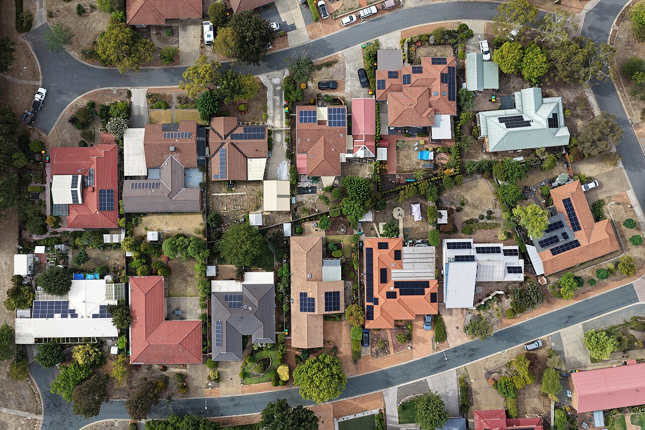
Figure 2: High-resolution aerial orthomosaic documenting the spatial density and orientation clustering of distributed rooftop solar photovoltaic arrays across residential and commercial buildings.
Desktop GIS & Python Rooftop Extraction Workflows
Deriving rooftop solar capacity across an entire municipal territory requires automated extraction of building roof planes, tilt angle calculation, aspect classification, and shading occlusion modeling.
1. Extracting Normalized Digital Surface Models (nDSM) in GDAL
Building heights and roof geometries are isolated by subtracting a bare-earth Digital Terrain Model (DTM) from a LiDAR first-return Digital Surface Model (DSM):
# Calculate normalized Digital Surface Model (nDSM) isolating above-ground structures
gdal_calc.py -A /data/dsm_lidar.tif -B /data/dtm_lidar.tif \
  --outfile=/data/ndsm_heights.tif \
  --calc="numpy.maximum(A - B, 0.0)" --NoDataValue=-9999

# Compute roof slope in degrees from the DSM
gdaldem slope /data/dsm_lidar.tif /data/roof_slope.tif -of GTiff

# Compute roof aspect in degrees (0 = North, 90 = East, 180 = South, 270 = West)
gdaldem aspect /data/dsm_lidar.tif /data/roof_aspect.tif -of GTiff -zero_for_flat
2. Python GeoPandas Rooftop Solar Yield Pipeline
The following automated Python pipeline reads building cadastral polygons, computes zonal statistics on roof slope and aspect, filters out unsuitable planes, and calculates installed peak capacity ($kW_p$) and annual yield ($MWh$):
import geopandas as gpd
import rasterio
from rasterstats import zonal_stats

def analyze_municipal_solar_capacity(cadastre_geojson, ndsm_raster, slope_raster, aspect_raster):
    """
    Computes usable rooftop PV capacity and estimated annual generation
    for municipal building cadastral footprints.
    """
    # 1. Load cadastral building footprints in projected CRS (e.g., EPSG:32633)
    gdf = gpd.read_file(cadastre_geojson)
    gdf["gross_area_m2"] = gdf.geometry.area

    # 2. Extract mean building height from nDSM
    stats_height = zonal_stats(gdf, ndsm_raster, stats="mean")
    gdf["building_height_m"] = [s["mean"] if s["mean"] else 0.0 for s in stats_height]

    # Filter out sheds and low fences (< 2.5 meters height)
    gdf = gdf[gdf["building_height_m"] >= 2.5].copy()

    # 3. Extract slope and aspect zonal metrics
    stats_slope = zonal_stats(gdf, slope_raster, stats="mean")
    stats_aspect = zonal_stats(gdf, aspect_raster, stats="mean")

    gdf["roof_slope_deg"] = [s["mean"] if s["mean"] else 0.0 for s in stats_slope]
    gdf["roof_aspect_deg"] = [s["mean"] if s["mean"] else 180.0 for s in stats_aspect]

    # 4. Apply suitability filters:
    # Reject steep slopes (> 45 deg) and direct north-facing roofs (aspect < 45 or aspect > 315)
    suitable_mask = (gdf["roof_slope_deg"] <= 45.0) & ~((gdf["roof_slope_deg"] > 10.0) & ((gdf["roof_aspect_deg"] < 45.0) | (gdf["roof_aspect_deg"] > 315.0)))
    gdf = gdf[suitable_mask].copy()

    # 5. Engineering Photovoltaic Calculations:
    # Usable packing factor = 0.70 (residential) to 0.60 (commercial)
    # Module efficiency = 20.5% at STC (0.205)
    # Regional irradiance = 1,650 kWh/m2/yr (Southern European / Mediterranean solar basin)
    # Performance ratio PR = 0.78
    usable_factor = 0.70
    eff = 0.205
    irradiance = 1650.0
    pr = 0.78

    gdf["net_solar_area_m2"] = gdf["gross_area_m2"] * usable_factor
    gdf["peak_capacity_kwp"] = gdf["net_solar_area_m2"] * eff
    gdf["annual_yield_mwh"] = (gdf["peak_capacity_kwp"] * irradiance * pr) / 1000.0
    gdf["co2_offset_tons"] = (gdf["annual_yield_mwh"] * 1000.0 * 0.380) / 1000.0

    print(f"Total Evaluated Buildings: {len(gdf)}")
    print(f"Total Potential Peak Capacity: {gdf['peak_capacity_kwp'].sum():,.1f} kWp ({gdf['peak_capacity_kwp'].sum()/1000:,.2f} MWp)")
    print(f"Total Annual Electricity Yield: {gdf['annual_yield_mwh'].sum():,.1f} MWh/year")

    # Export prioritized municipal solar geodatabase
    gdf.to_file("/data/municipal_solar_potential.geojson", driver="GeoJSON")
    return gdf
Common Pitfalls and Field Troubleshooting in Rooftop PV
Discrepancies between projected preliminary estimates and real operational energy yields stem from practical physical constraints that are frequently neglected during early GIS desktop assessments:
1. Gross Envelope Overestimation and Rooftop Obstacles
Commercial and industrial rooftops are rarely clear open planes. In practical inspections, rooftop surface area is obstructed by:
- HVAC rooftop chillers, air handling units, and condenser fans.
- Skylights, translucent daylight panels, and smoke evacuation hatches.
- Drainage valleys, internal gutters, and fire protection parapets.
- Mandatory fire department perimeter access corridors (typically 1.5 to 2.0 meters wide).
Applying an unadjusted gross area directly into a yield formula overestimates actual DC capacity by 30% to 50%. On flat commercial roofs, a packing factor between 0.55 and 0.65 must be applied to account for required inter-row maintenance corridors and shade-avoidance pitch spacing.
2. Inverter Sizing, Clipping, and DC-to-AC Inverter Loading Ratio (ILR)
System designers frequently oversize DC array capacity relative to inverter AC nameplate capacity (e.g., $1.25\text{ kWp DC}$ per $1.0\text{ kW AC}$ inverter rating, yielding an $ILR = 1.25$). While this oversizing maximizes inverter capacity factor during morning, late afternoon, and cloudy winter hours, it induces inverter power clipping during bright summer midday peaks.
If the DC array capacity exceeds the maximum input voltage or current thresholds of the inverter, the inverter shifts its maximum power point tracking (MPPT) voltage away from $V_{mpp}$ to throttle power intake. Modeling software that assumes linear inverter scaling without clipping limits will overestimate summer generation by 2% to 6%.
3. High-Voltage Distribution Grid Hosting Bottlenecks
In rural or suburban areas with high agricultural warehouse penetration (such as high-density agricultural solar corridors and rural industrial zones), local distribution circuits can become saturated with solar power during sunny hours. When concurrent local generation exceeds local transformer substation capacity, reverse power flows toward the transmission grid cause distribution line voltages to rise.
Grid operators mandate that solar inverters trip offline or throttle output when line voltage exceeds statutory limits (e.g., $+10\%$ above nominal 400 V / 230 V). Facilities experiencing chronic voltage-trip shutdowns suffer severe revenue losses despite pristine meteorological solar resource availability.
4. Parapet Shading and Micro-Topography
Flat roofs surrounded by 1.0 to 1.5-meter masonry parapets cast substantial horizontal shadows early in the morning and late in the afternoon. Because modern crystalline modules are connected in series strings, shading a single cell along the southern or eastern perimeter drops the operating current of the entire string to near zero. A 2-meter buffer setback from all perimeter parapets must be enforced in the GIS layout plan.
Frequently Asked Questions on Rooftop Solar PV Capacity
What is the physical meaning of the Photovoltaic Performance Ratio (PR)?
The Performance Ratio (PR) is a dimensionless metric defined by IEC 61724 that quantifies the overall optical, thermal, and electrical efficiency of a photovoltaic plant relative to its nominal nameplate capacity at Standard Test Conditions (STC). A PR of 0.78 indicates that 78% of the incident solar energy theoretically convertible at STC is actually delivered as alternating current (AC) to the grid, with 22% dissipated through thermal derating, inverter clipping, DC/AC cable resistance, soiling, and module mismatch.
Why is the usable roof factor typically lower on flat commercial roofs than on sloped residential roofs?
Flat commercial roofs require modular racking tilted toward the equator. To prevent the front row of modules from casting shadows onto trailing rows during low winter sun angles, generous inter-row pitch spacing is required. Furthermore, commercial roofs host rooftop HVAC chillers, smoke vents, access pathways, and perimeter fire safety setbacks, reducing net usable surface fraction to 55% - 65%. In contrast, pitched residential roofs allow coplanar flush mounting across up to 75% - 85% of an equator-facing plane.
How does extreme ambient summer heat reduce the power output of monocrystalline solar modules?
Silicon photovoltaic cells lose efficiency as junction temperature increases. The temperature coefficient of maximum power (gamma_pmax) for modern monocrystalline PERC and TOPCon modules ranges between -0.30% and -0.38% per degree Celsius above the 25 deg C STC reference. In summer ambient conditions of 38 deg C with high irradiance, rooftop cell operating temperatures can reach 65 deg C (a 40 deg C rise), causing an immediate instantaneous power derate of 12% to 15%.
What criteria distinguish Low Tension (BT) from Medium Tension (MT) grid interconnections in European power grids?
Under European distribution grid standards (such as EN 50549 and CEI specifications), installations with peak capacity under 200 kW connect directly to the Low Voltage three-phase distribution network (400 V LV / BT). Facilities between 200 kW and 5,000 kW (5 MW) require a dedicated pad-mounted step-up transformer and connect to the Medium Voltage distribution network (15 kV to 20 kV MV / MT). Utility plants exceeding 5 MW connect directly to the High Voltage transmission grid (150 kV HV / AT).
How is specific yield (kWh/kWp/year) used to evaluate the economic quality of a solar site?
Specific yield normalizes total annual kilowatt-hour energy generation by installed peak DC capacity (Annual Generation in kWh / Peak Power in kWp). It reflects the local solar resource and system efficiency independent of installation size. In northern Europe, specific yield averages 900 to 1,150 kWh/kWp/year, while in Mediterranean solar basins across Southern Europe (including Spain, Italy, and Greece), specific yield reaches 1,400 to 1,650 kWh/kWp/year.