Spectral Index & Band Math Calculator
Client-side Earth observation band math engine. Evaluate spectral transformations across vegetation, water, urban built-up, and soil sealing indices with homologous Sentinel-2 and Landsat band mappings, threshold segmentation, and automated code recipes.
Theoretical and Mathematical Foundation
Spectral indices constitute one of the most computationally efficient and interpretable approaches for extracting land-use and land-cover (LULC) information from satellite observations. By formulating mathematical ratios or normalized differences between specific spectral bands, indices exploit the differential absorption and reflectance properties of terrestrial materials to enhance target signals while suppressing background noise.
The Bare Soil vs Impervious Surface Challenge
While identifying dense vegetation (using NDVI) or open water bodies (using NDWI or MNDWI) is straightforward due to their distinctive absorption signatures, the automated discrimination of sealed urban surfaces (asphalt, concrete, rooftop materials) from exposed bare mineral soils represents one of remote sensing's most persistent challenges.
At medium spatial resolutions (10 to 30 meters), individual pixels frequently contain complex sub-pixel mixtures of artificial impervious materials, bare compacted ground, and sparse dry vegetation. In arid and semi-arid regions, as well as during dry summer months in temperate zones, the moisture content of exposed agricultural soils decreases significantly. Because water absorption in the Shortwave Infrared (SWIR) region is progressively attenuated as soil dries, dry soils exhibit a pronounced spectral rise from visible wavelengths into the SWIR domain:
Impervious Urban Signature: Low-to-Moderate Visible -> Moderate NIR -> Elevated SWIR1 & SWIR2
Classical urban indices, including the Normalized Difference Built-up Index (NDBI) and the New Built-up Index (NBI), rely primarily on the contrast between SWIR1 and NIR:
NBI = (SWIR1 * Red) / NIR
Because both dry mineral soils and artificial construction materials display elevated SWIR1 relative to NIR, NDBI and NBI generate high positive values for both classes, leading to substantial commission errors where plowed fields, construction sites, and fallow lands are erroneously classified as urban soil sealing.
Mathematical Derivation of the Sealed Urban Index (SUI)
To resolve this spectral ambiguity without requiring computationally intensive machine learning models or region-specific training data, the Sealed Urban Index (SUI) (Asad, Capolupo & Tarantino, 2025) combines two normalized spectral contrasts derived from the visible and shortwave infrared regions:
The formulation relies on two normalized components:
C_2 = (SWIR2 - Red) / (SWIR2 + Red)
The first component, C_1, captures the relative contrast between the visible green band and SWIR1. In sealed urban surfaces, SWIR1 reflectance consistently exceeds Green reflectance, producing negative values for (Green - SWIR1). Bare soils exhibit a wider distribution depending on mineralogy and organic matter content.
The second component, C_2, characterizes the spectral slope between the Red visible band and SWIR2. Dry mineral soils generally display a steeper increase in reflectance extending all the way into SWIR2, whereas artificial urban materials display a different, flatter spectral trajectory across this longer wavelength interval.
The Multiplicative Interaction as a Joint Spectral Constraint
The structural hallmark of SUI is its non-linear multiplicative interaction: C_1 * C_2. In traditional additive or linear combinations (e.g. C_1 + C_2), a very strong response in one spectral component can compensate for a weak or contradictory response in the other component, resulting in a high index score even when only one physical condition is satisfied. This compensation effect is particularly problematic in mixed pixels along urban fringes.
The multiplicative structure suppresses this compensation effect. High positive product values are obtained only when both normalized contrasts consistently exhibit the spectral configuration characteristic of sealed surfaces. The multiplicative interaction acts as a strict joint constraint, increasing target selectivity and attenuating ambiguous responses from mixed pixels. Finally, the additive constant (+0.5) shifts the resulting index distribution into a positive range, establishing stable decision thresholds:
Multi-Temporal Change Detection & Feature-Space Separability
In multi-temporal change detection frameworks, single-date spectral thresholding is strengthened by vector-space trajectory analysis. When monitoring urban expansion and soil sealing across successive satellite acquisitions (from time t_1 to time t_2), feature vectors combining multi-temporal spectral bands and indices are projected into an n-dimensional metric space.
The degree of spectral transformation is evaluated using the Cosine Distance metric:
D_cos(u, v) = 1 - ( (u . v) / ( ||u||_2 * ||v||_2 ) )
Cosine distance measures the angular displacement between multi-spectral vectors rather than Euclidean magnitude, making it robust against atmospheric lighting variations, sun angle shifts, and sensor calibration drifts. Stable land cover types (such as persistent forest canopy, water bodies, and established urban infrastructure) cluster tightly at minimal cosine distances. Conversely, abrupt land transformation events (such as the conversion of natural soil or agricultural fields into asphalt surfaces, warehouse concrete slabs, and industrial pads) manifest as significant angular vector shifts. Setting a calibrated empirical decision threshold effectively separates permanent anthropogenic soil consumption from seasonal crop phenology cycles and transient soil moisture variations.

Figure 1: Bottom-of-Atmosphere (BOA) surface reflectance profiles across the solar reflective spectrum, illustrating the distinctive spectral curves of healthy green vegetation, bare mineral soil, impervious urban surfaces, and clear water relative to Sentinel-2 MSI bands.
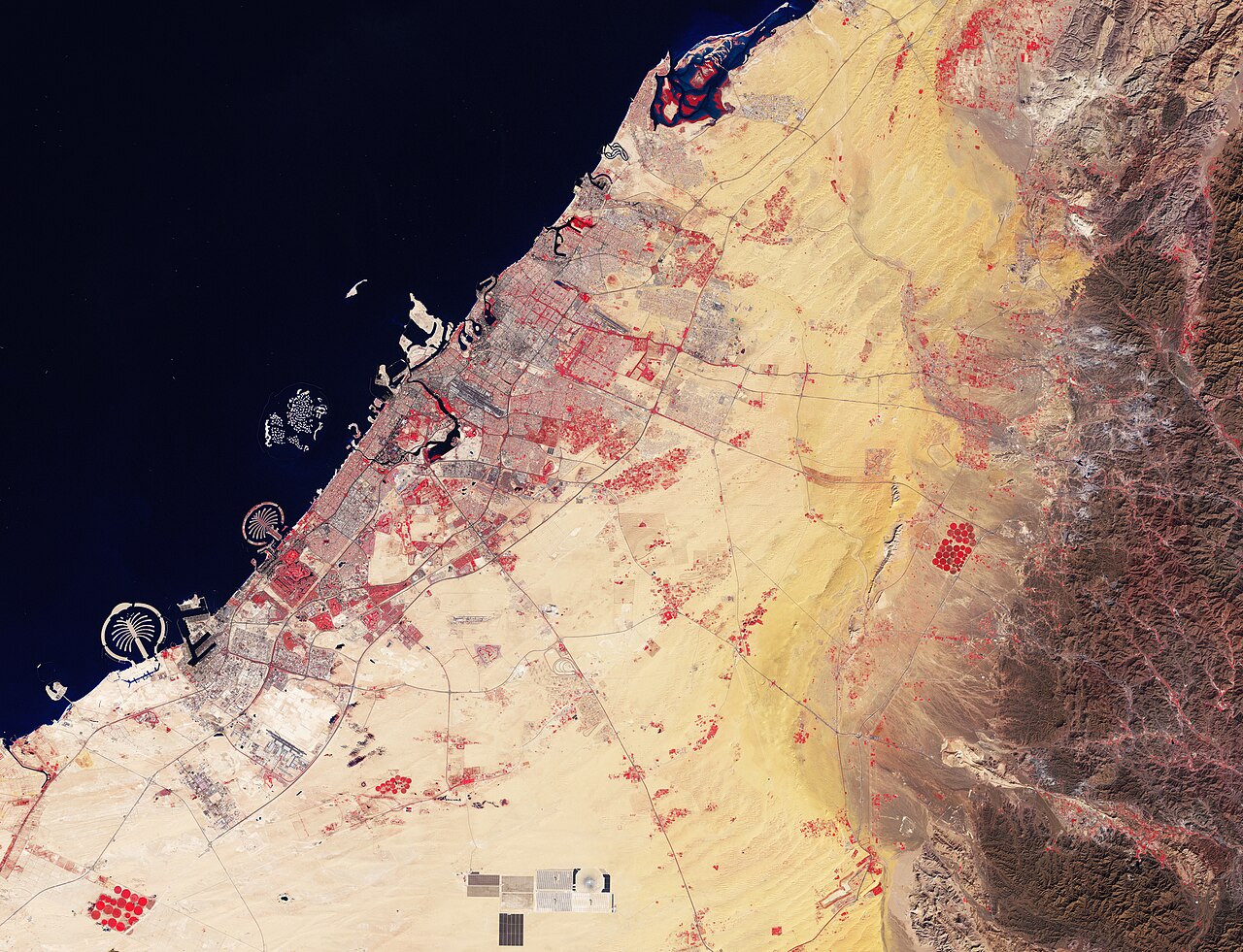
Figure 2: Copernicus Sentinel-2 Level-2A false-color infrared visualization, highlighting the sharp spectral demarcation between densely sealed urban infrastructure, open water bodies, and surrounding vegetated land cover.
Applying a calibrated vector distance threshold filters out seasonal crop phenology noise and bare soil moisture variations while capturing true anthropogenic soil consumption.
| Satellite Sensor | Homologous Bands Used | Optimal Classification Threshold | Validation F1-Score (Sealed Class) | Overall Accuracy (OA) |
|---|---|---|---|---|
| Sentinel-2 MSI (10-20m) | B03 (Green), B04 (Red), B11 (SWIR1), B12 (SWIR2) | Threshold >= 0.47 | 0.74 to 0.80 | 82.6% to 87.0% |
| Landsat 8-9 OLI (30m) | B3 (Green), B4 (Red), B6 (SWIR1), B7 (SWIR2) | Threshold >= 0.46 | 0.71 to 0.76 | 78.9% to 82.4% |
Step-by-Step Desktop GIS and Command-Line Workflow
The workflows below illustrate how to calculate SUI and standard spectral indices across QGIS Desktop, Google Earth Engine, and standalone Python pipelines.
Calculating SUI in QGIS Raster Calculator
- Load Harmonized Bands: Import Sentinel-2 Level-2A surface reflectance bands:
B03(Green),B04(Red),B11(SWIR1), andB12(SWIR2). Ensure 20m bands (B11, B12) are resampled to 10m. - Open Calculator: Select Raster -> Raster Calculator.
- Enter Formula with Denominator Clamping: Enter the following formula into the expression window:
((( "B03@1" - "B11@1" ) * ( "B12@1" - "B04@1" )) / (( "B03@1" + "B11@1" + 0.000001 ) * ( "B12@1" + "B04@1" + 0.000001 ))) + 0.5 - Segment Impervious Surfaces: In the raster calculator, threshold the SUI raster to extract binary soil sealing:
The resulting binary raster displays 1 for sealed surfaces and 0 for non-sealed surfaces.
"SUI@1" >= 0.47
Google Earth Engine (GEE) Production Script
The complete GEE implementation below includes cloud masking, bilinear resampling of 20m bands to 10m, epsilon denominator clamping, and threshold classification:
// 1. Cloud Masking using Scene Classification Layer (SCL)
function maskS2Clouds(image) {
  var scl = image.select('SCL');
  // Mask out saturated pixels (1), dark cast shadows (2), cloud shadows (3),
  // medium/high probability clouds (8, 9), cirrus (10), and snow/ice (11)
  var mask = scl.neq(1).and(scl.neq(2)).and(scl.neq(3))
    .and(scl.neq(8)).and(scl.neq(9)).and(scl.neq(10)).and(scl.neq(11));
  return image.updateMask(mask);
}

// 2. Resample 20m SWIR bands to 10m via bilinear interpolation
function resampleTo10m(image) {
  return image.resample('bilinear').reproject({
    crs: image.select('B2').projection(),
    scale: 10
  });
}

// 3. Compute Sealed Urban Index with Epsilon Safeguard
function computeSUI(image) {
  var green = image.select('B3').divide(10000.0);
  var red = image.select('B4').divide(10000.0);
  var swir1 = image.select('B11').divide(10000.0);
  var swir2 = image.select('B12').divide(10000.0);

  var eps = ee.Image(1e-6);
  var denom1 = green.add(swir1).max(eps);
  var denom2 = swir2.add(red).max(eps);

  var sui = green.subtract(swir1)
    .multiply(swir2.subtract(red))
    .divide(denom1.multiply(denom2))
    .add(0.5)
    .rename('SUI');

  var sealedMask = sui.gte(0.47).rename('Sealed_Surfaces');
  return image.addBands([sui, sealedMask]);
}

// Map workflow over region of interest
var dataset = ee.ImageCollection('COPERNICUS/S2_SR_HARMONIZED')
  .filterBounds(roi)
  .filterDate('2024-01-01', '2024-12-31')
  .filter(ee.Filter.lt('CLOUDY_PIXEL_PERCENTAGE', 10))
  .map(maskS2Clouds)
  .map(resampleTo10m)
  .map(computeSUI);

var medianComposite = dataset.median();
Map.addLayer(medianComposite.select('SUI'), {min: 0.3, max: 0.6, palette: ['blue', 'yellow', 'red']}, 'SUI Index');
Map.addLayer(medianComposite.select('Sealed_Surfaces'), {min: 0, max: 1, palette: ['black', 'red']}, 'Sealed Binary');
Python Vectorized Array Script with Rasterio
import rasterio
import numpy as np

def compute_sui_raster(green_path, red_path, swir1_path, swir2_path, out_path):
    with rasterio.open(green_path) as src_g:
        meta = src_g.meta.copy()
        green = src_g.read(1).astype('float32') / 10000.0

    with rasterio.open(red_path) as src_r:
        red = src_r.read(1).astype('float32') / 10000.0

    with rasterio.open(swir1_path) as src_s1:
        swir1 = src_s1.read(1).astype('float32') / 10000.0

    with rasterio.open(swir2_path) as src_s2:
        swir2 = src_s2.read(1).astype('float32') / 10000.0

    eps = 1e-6
    denom1 = np.maximum(green + swir1, eps)
    denom2 = np.maximum(swir2 + red, eps)

    c1 = (green - swir1) / denom1
    c2 = (swir2 - red) / denom2
    sui = (c1 * c2) + 0.5

    # Binary classification threshold
    sealed_mask = (sui >= 0.47).astype('uint8')

    meta.update({'dtype': 'uint8', 'count': 1, 'compress': 'deflate'})
    with rasterio.open(out_path, 'w', **meta) as dst:
        dst.write(sealed_mask, 1)

print(f"Classification successfully written to {out_path}")Common Pitfalls and Field Troubleshooting
Computing spectral indices across extensive territorial mosaics exposes algorithms to edge-case reflectance conditions. The primary operational pitfalls are detailed below.
1. Denominator Collapse and Zero-Division Exceptions
In clear deep water bodies, mountain shadows, or cloud shadow masks, surface reflectance in the visible green and SWIR channels frequently drops close to 0.000. Without numerical clamping:
In Google Earth Engine, division by zero results in unmasked null pixels. In Python NumPy arrays, it produces NaN or Inf values that disrupt downstream statistical aggregations. Imposing an epsilon lower bound (ε = 1e-6) ensures that all operations return finite, mathematically stable values without perturbing valid physical reflectance numbers.
2. Digital Number Scale Factor Neglect
A frequent data engineering mistake is applying spectral index equations directly to raw Digital Numbers (DN) stored in integer files. If an analyst enters raw Sentinel-2 DN values (e.g. Green = 850, SWIR1 = 2100):
While normalized ratios are theoretically scale-invariant, any formula that incorporates additive offsets (such as SUI's +0.5) will produce incorrect results if digital numbers are not divided by 10,000 first.
3. Spatial Allocation Disagreement vs Quantity Disagreement
When validating index-based classifications against ground truth points, analysts often focus exclusively on Overall Accuracy (OA). However, Pontius and Millones (2011) demonstrate that classification disagreement consists of two independent components: Quantity Disagreement (QD) and Allocation Disagreement (AD).
| Error Component | Physical Meaning | Observed Empirical Value | Engineering Interpretation |
|---|---|---|---|
| Quantity Disagreement (QD) | Error in total class area estimation | 0.003 to 0.019 (Very Low) | The index reliably estimates the total regional surface area of soil sealing with negligible bias. |
| Allocation Disagreement (AD) | Error in spatial pixel placement | 0.130 to 0.200 (Moderate) | Errors are concentrated along heterogeneous boundaries where 10-30m pixels contain mixed land cover. |
Because QD remains minimal across multi-year trials, SUI is highly dependable for aggregate municipal soil sealing accounting, while fine boundary delineation benefits from object-based post-processing or machine learning integration.
Frequently Asked Questions
How does the SUI threshold behave across arid climates like North Africa?
In arid and semi-arid environments (such as North Africa), extreme soil dryness increases bare soil SWIR reflectance. Empirical optimization reveals that the optimal threshold shifts slightly lower (mean 0.46 for Sentinel-2, 0.45 for Landsat). However, the performance plateau around 0.47 is broad, meaning a global threshold of 0.47 yields stable, transferable accuracy without requiring site-specific retraining.
Can SUI be calculated from airborne UAV or drone multispectral cameras?
Standard commercial drone multispectral sensors (such as the DJI Mavic 3 Multispectral or MicaSense RedEdge) typically include Blue, Green, Red, Red Edge, and Near Infrared bands, but lack Shortwave Infrared (SWIR-1 and SWIR-2) detectors due to detector cooling constraints. Because SUI requires SWIR bands (centered near 1.6 and 2.2 micrometers), it cannot be computed from basic VNIR drone sensors. For drone sensors, indices such as the Visible Atmospherically Resistant Index (VARI) or high-resolution spatial texture metrics are used.
Why is annual median compositing preferred over single-date satellite imagery?
Single-date satellite imagery is subject to transient atmospheric noise, temporary agricultural plowing, seasonal phenological flushes, and localized cloud shadows. Computing the annual pixel-wise median across all cloud-free observations eliminates short-term outliers, suppresses transient agricultural bare soil states, and provides a representative surface reflectance baseline that reflects permanent land-cover transformations.
How does machine learning (CART or SVM) enhance single-index classification?
While threshold-based classification applies a single scalar boundary across one index, machine learning algorithms like Support Vector Machines (SVM) and Classification and Regression Trees (CART) map a multi-dimensional feature space integrating multiple indices (SUI, BLFEI, BRBA, NBI, BUI, Fe) alongside raw spectral bands. In empirical evaluations, SVM with multi-index features achieved overall accuracies exceeding 90% across diverse climatic regions by modeling non-linear class boundaries in complex transitional zones.
What is the Ferric Oxide Index (Fe) used for in land-cover analysis?
The Ferric Oxide Index (Fe = Red / Blue) detects iron oxide minerals (hematite, goethite) that exhibit strong blue absorption and elevated red reflectance. In urban and peri-urban mapping, it helps identify terracotta tile roofs, weathered brick masonry, and iron-rich degraded soils, providing complementary discriminatory evidence when combined with built-up indices.